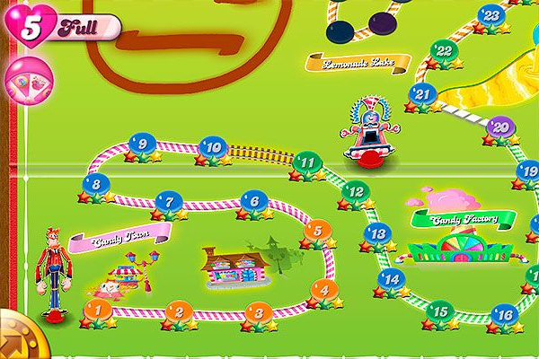
Level Balancing: Game Difficulty data-driven adjustments in Candy Crush
Abstract: This study explores the impact of game difficulty on player engagement within mobile Puzzle Games, positing that the level of challenge significantly influences player retention and satisfaction. Utilizing Python and Plotly for data preprocessing and visualization, the study analyzes player attempts and success rates across various levels, based on a dataset provided by Rasmus Baath. The findings reveal a generally well-balanced difficulty spectrum, advocating for the implementation of dynamic difficulty adjustments to optimize engagement. The conclusion underscores the importance of maintaining diverse difficulty levels to minimize player attrition, highlighting a subset of levels that pose exceptional challenges.
⚠️ Introduction to problem
Hypothesis
We’ll review a game that potentially can lead any developer to many unseen problems, considering the abundance of levels. From the perspective of a customer, there can be several points of view that can emerge and, at the same time, can become unnoticed. That’s why our diagnosis will start from 2 potential hypothesis:
- $H_0:$ The game is too easy so it became boring over time.
- $H_1:$ The game is too hard so the players leave it and become frustrated.
Potential Stakeholders
None of the past hypotheses are the main intentions of the developers. So they require a Data Analyst to help with this task since the developers are seeing only the backend factors affecting the game, but it’s also critical to consider those external ones that affect the experience for the player and the sustainability of this game for the company. Among the main stakeholders could be:
- Level Designers: They work aligned with the rest of the Engineering Team because they still have a backend perspective and their next patch release needs to be aligned with the insights given by the analyst.
- Mobile Designer & User Retention Expert: This is a game whose main income input is in-game purchases because it’s a F2P, the main source of income is centered in retain the engagement in the game and keeping the consumers on the platform.
- Gameplay Engineer: They require to start working on the difficulty adjustment patch as soon as they receive the final statement.
- Executive Producer: Besides Candy Crush being an IP with internal producers since it’s developed and published by King, the parent company will expect to have an ROI aligned with their expectations.
- Players' community: They expect to have an endurable and great experience with a brief response in case of disconformities.
Note: To facilitate the understanding of the roles of the development team, I invite you to take a look at this diagram that I designed.
📥 About the data
Collection process and structure
Before start let’s import the libraries we’re going to need
|
|
Due to the extensive size of possible episodes to analyze, we’ll limit the analysis to just one of them, which exactly will have data available for 15 levels. To do this, the analysts need to request a sample from the telemetry systems to get data related to the number of attempts per player in each episode level.
Also, it’s important to mention that in terms of privacy, this analysis requires importing the data with the player_id codified for privacy reasons. Fortunately, in this case, Rasmus Baath, Data Science Lead at castle.io, provided us with a Dataset with a sample gathered in 2014.
|
|
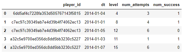
We can see that our data is structured and consists of 5 attributes:
- player_id: a unique player id
- dt: the date
- level: the level number within the episode, from 1 to 15
- num_attempts: number of level attempts for the player on that level and date
- num_success: number of level attempts that resulted in a success/win for the player on that level and date
🔧 Data Preprocessing
Before starting the analysis we need to do some validations on the dataset.
|
|
|
|
Data Cleaning
The data doesn’t require any kind of transformation and the data types are aligned with their purpose.
|
|
|
|
Data Consistency
The usability of the data it’s rather good, since we don’t count with “NAN” (Not A Number), “NA” (Not Available), or “NULL” (an empty set) values.
|
|
|
|
By this way, we can conclude that there were not errors in our telemetry logs during the data collection.
Normalization
Next, we can conclude there were no impossible numbers, except for a player that tried to complete the level 11 in 258 attempts with just 1 success. This is the only registry we exclude since it can be an influential outlier and we don’t rely on more attributes about him to create conclusions.
Noticing the distribution of the quartiles and comprehending the purpose of our analysis, we can validate that the data is comparable and doesn’t need transformations.
|
|
🔍 Exploratory Analysis & In-game interpretations
Summary statistics
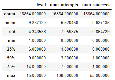
Excluding the outliers we mentioned before, we got the next conclusions about their distribution and measurement:
- player_id
- Interpretation: Not unique and counts with 6814 distinct values which make sense since there is a player with records of multiple levels
- Data type: Nominal
- Measurement type: Discrete/String
- dt
- Interpretation: Only includes data from January 1st to January 7th of 2014. Also, the analysis won’t consider this as a lapse per player since the records per player are not continuous, so they will be limited as a timestamp
- Data type: Ordinal
- Measurement type: Temporal
- level
- Interpretation: They’re registered as numbers, but for further analysis will be transformed as factors. 50% of the records are equal to or less than level 9
- Data type: Ordinal
- Measurement type: Discrete/String
- num_attempts
- Interpretation: The registries are consistent, the interquartile range mention that half of the players try between 1 and 7 time to complete each level. Furthermore, there are players with 0 attempts, so we need to evaluate if this is present at level 1, which can explain a problem in retention rate for that episode
- Data type: Numerical
- Measurement type: Integer
- num_success
- Interpretation: Most of the players are casual gamers because 75% of them complete the level and don’t repeat it
- Data type: Numerical
- Measurement type: Integer
Levels played in Episode
First, let’s examine the number of registries per player.
This will tell us, from the episode how many levels have each player recorded in the lapse of 7 days.
|
|
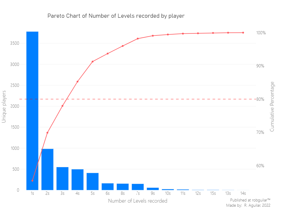
From the last Pareto chart, we can deduce that 80% of the 6814 players just count with 3 levels recorded of 15. But, since this was extracted from a random sample, this won’t affect our study.
Difficulty of completing a level in a single try
There is a combination of easier and challenging levels. Chance and skills make the number of attempts required to pass a level different from one player to another. The presumption is that difficult levels demand more tries on average than easier ones. That is, the harder a level is the lower the likelihood to pass that level in a single try.
In these circumstances, the Bernoulli process might be useful. As a Boolean result, there are only two possibilities, win or lose. This can be measured by a single parameter:
$p_{win} = \frac{\Sigma wins }{\Sigma attempts }$: the probability of completing the level in a single attempt
Let’s calculate the difficulty $p_{win}$ individually for each of the 15 levels.
|
|
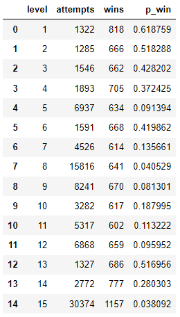
We have levels where 50% of players finished on the first attempt and others that are the opposite. But let’s visualize it through the episode, to make it clear.
|
|
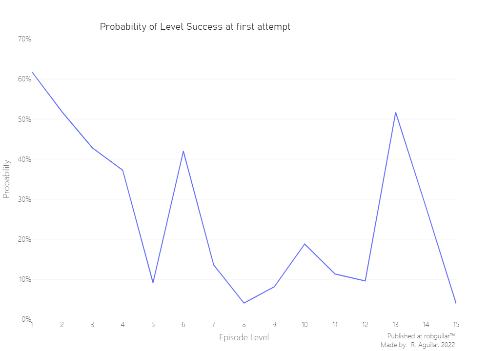
Defining hard levels
It’s subjective what we can consider a hard level because not consistently depends on a single factor and for all player profile groups this can be different. So, for the outcomes of this study, we will arbitrarily assume that a difficult level is the one that has a probability to be completed in the first attempt of a 10% ($p_{win} < 10%$).
|
|
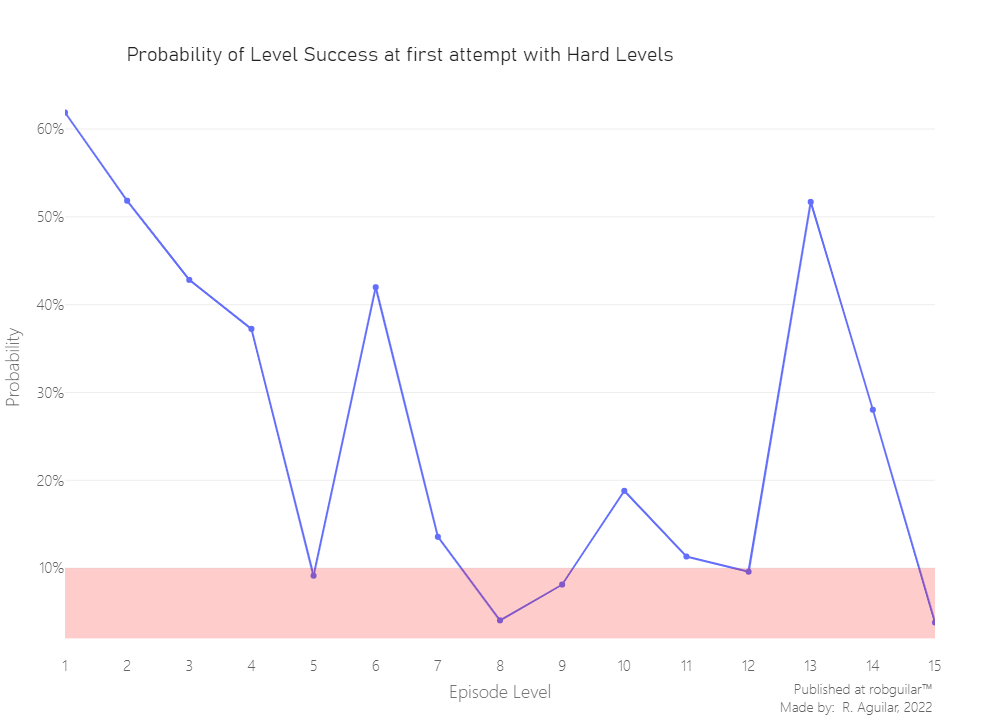
From our predefined threshold, we see that the level digit is not aligned with its difficulty. While we have hard levels as 5, 8, 9, and 15; others like 13 and 15 are unleveraged and need to be rebalanced by the level designers.
Measuring the uncertainty of success
We should always report some calculation of the uncertainty of any provided numbers. Simply, because another sample will give us little different values for the difficulties measured by level.
Here we will simply use the Standard error as a measure of uncertainty:
$\sigma_{error} \approx \frac{\sigma_{sample}}{\sqrt{n}}$
Here n is the number of datapoints and $\sigma_{sample}$ is the sample standard deviation. For a Bernoulli process, the sample standard deviation is:
$\sigma_{sample} = \sqrt{p_{win}(1-p_{win})}$
Therefore, we can calculate the standard error like this:
$\sigma_{error} \approx \sqrt{\frac{p_{win}(1-p_{win})}{n} }$
Consider that every level has been played n number of times and we have their difficulty $p_{win}$. Now, let’s calculate the standard error for each level of this episode.
|
|
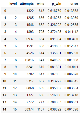
We have a measure of uncertainty for each levels' difficulty. As always, this would be more appealing if we plot it.
Let’s use error bars to show this uncertainty in the plot. We will set the height of the error bars to one standard error. The upper limit and the lower limit of each error bar should be defined by:
$p_{win} \pm \sigma_{error}$
|
|
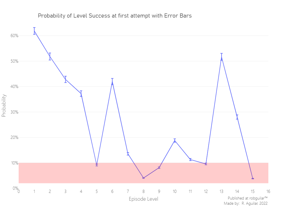
Looks like the difficulty estimates a very exact. Furthermore, for the hardest levels, the measure is even more precise, and that’s a good point because from this we can make valid conclusions based on that levels.
As a curious fact, also we can measure the probability of completing all the levels of that episode in a single attempt, just for fun.
|
|
|
|
🗒️ Final thoughts & takeaways
What can the stakeholders understand and take into consideration?
From the sample extracted we conclude that just 33% of the levels are considered of high difficulty, which it’s acceptable since each episode counts with 15 levels, so by now the level designer should not worry about leveling the difficulty.
What could the stakeholders do to take action ?
As a suggestion, in the case that the Publisher decides to invest more in in-game mechanics, a solution for a long-time and reactive engagement could be the use of Machine Learning to generate a DGDB as some competitors have adapted in IPs like EA Sports FIFA, Madden NFL or the “AI Director” of Left 4 Dead.
What can stakeholders keep working on?
The way their level difficulty design work today is precise since our first hypothesis was that the game wasn’t too linear to unengaged the player and churn as consequence. Because as we saw, the game has drastic variations in the levels 5-6 and 8-10, which can help to avoid frustrations in players.
ℹ️ Additional Information
- About the article
Based on the dataset provided, we will not proceed with a retention analysis as mentioned above. Because the data is from a random episode, if this were episode one, this type of analysis could be useful as it can explain the pool of players who log in, created an account, or install the game but never start playing, causing traction problems. Therefore, this will be left as a limitation to the scope of the analysis.
With acknowledgment to Rasmus Baraath for guiding this project. Which was developed for sharing knowledge while using cited sources of the material used.
Thanks to you for reading as well.
- Related Content
— Rasmus Baath personal blog
— Anders Drachen personal website
- Datasets
This project was developed with a dataset provided by Rasmus Baraath, which also can be downloaded at my Github repository.