Optimizing User Retention in Brawl Stars: Unsupervised Machine Learning Approach to Cohorts Retention Metrics

2023-05-20 9840 words 47 minutes

Contents

Abstract: This study presents a comprehensive investigation into the development of a player retention pipeline and the establishment of user cohorts for the game Brawl Stars through the application of unsupervised machine learning models. The primary aim is to enhance the analysis of user retention by implementing advanced cohort classification techniques and the generation of retention metrics. To achieve this, the research utilizes data obtained from the Brawl Stars public API, applies KMeans clustering for the categorization of players, and employs PySpark for data processing and analysis, with an emphasis on the use of Kedro for the efficient assembly of the data processing pipeline. The outcomes of this analysis underscore the pipeline’s proficiency in handling vast datasets and augmenting the production of retention metrics. The results suggest that this automated strategy provides clear insights into player behaviors and retention rates, endorsing its integration into game development practices and its potential adaptability for Google Cloud Deployments.

Important: Any views, material or statements expressed are mines and not those of my employer, read the disclaimer to learn more.¹

Looking for an interactive experience?

🚀 Access the source code from GitHub

⚠️ Introduction to the problem

Hypothesis

The analytics team of a mobile gaming developer is facing a problem while producing bounded retention metrics for player cohorts based on the game modes offered. They need a fully parameterized way to produce these metrics, instead of hardcoded methods per iteration.

Currently, the analytics team mines data batches of over 20,000 players in a single run to create unbounded retention metrics, and the job is processed every 56 days. However, the team need to track user retention within a given time frame and qualify player preferences based on the game modes offered and their game-experience.

Also, they require a model that can define cohorts based on the installation date or any other classification parameter and includes a feature store to keep track of the features used. Additionally, they would like to store the hyperparameters, evaluation scores, and estimators used for each experiment on a Cloud Service to reuse specific models later.

$H_0:$ The pipeline is sufficient to produce retention metrics for player cohorts based on the game modes offered, and there is no need for a fully parameterized tool to create these metrics with bounded approaches.
$H_1:$ The current pipeline is not sufficient, and a fully parameterized tool is required to track user retention within a given time frame and qualify player preferences based on the game modes offered. Additionally, a Cloud Service-based feature store and model registry are needed to keep track of experiment versions.

Potential Stakeholders

Designers: Game Designers are interested in user retention metrics to understand how users are interacting with the game and to identify any areas that need to be improved to keep users engaged and coming back to the game.
Product / Project Managers: Responsible for defining the goals and objectives for the game and ensuring that those goals are met, they need to follow user retention metrics to understand how well the game is performing in terms of retaining users and whether any changes need to be made to the game to improve retention.
Marketer: Understand how effective their marketing campaigns are in “keeping users engaged” with the game, and whether any changes need to be made to the campaigns to improve retention.
Programmers: Interested in identifying any technical issues that may be causing users to leave the game and make improvements to the game to improve retention.
Publisher: Need to understand the financial performance of the game and whether it is generating sufficient revenue to justify the investment. They are also interested in understanding the potential for future growth and the impact of retention on the game’s long-term sustainability.

Note: To facilitate the understanding of the roles of the development team, I invite you to take a look at this diagram that I designed.

📥 About the data

Source data

The Brawl Stars Public API is the source of the data, which is accessible to anyone and completely free to use. By entering an identifier in the request function, the API gathers data on the player associated with that identifier, also known as the “Player Tag”.

Each user account has a unique player tag, which I collected from a sample shared by @SirWerto on Kaggle. To supplement our tag list, also utilized the .ranking() function of Brawlstats, an open-source Python library. The dataset contains a total of 23841 Player Tags, which are saved in a .txt file and stored in a Google Cloud Bucket folder labeled as /01_player_tags.

Data Catalog structure

Versioning plays a vital role in maintaining organized and traceable files. To accomplish this, we utilize a hierarchical storage approach, incorporating a timestamp in EPOCH format as a reference point. In order to leverage this functionality, we will employ the Kedro versioning feature.

To ensure a comprehensive record of models, estimators, and features used in each run, the catalog offers eight distinct storage endpoints, including /06_viz_data, /07_feature_store, and /08_model_registry, all of which are versioned. By using versioning to manage and maintain these files, teams can easily track data and model changes, to ensure that each iteration is saved for future reference.

 1
 2
 3
 4
 5
 6
 7
 8
 9
10
11
12
13


gcp:
    # ----- Bucket Parent Locations -----
    player_tags: gs://animus-memory-bucket/brawlstars/01_player_tags
    raw_battlelogs: gs://animus-memory-bucket/brawlstars/02_raw_battlelogs
    raw_metadata: gs://animus-memory-bucket/brawlstars/03_raw_metadata
    enriched_data: gs://animus-memory-bucket/brawlstars/04_enriched_data
    curated_data: gs://animus-memory-bucket/brawlstars/05_curated_data
    viz_data: gs://animus-memory-bucket/brawlstars/06_viz_data
    feature_store: gs://animus-memory-bucket/brawlstars/07_feature_store
    model_registry: gs://animus-memory-bucket/brawlstars/08_model_registry

    # ----- Main GCP Project ID -----
    project_id: abstergo-corp-id

To easily locate the endpoint of each GCP Bucket output, simply refer to the conf/gcp/catalog.yml file. This file defines each destination using Dataset Groups, as shown in the following example:

 1
 2
 3
 4
 5
 6
 7
 8
 9
10
11
12
13
14
15
16
17
18
19
20
21
22
23
24
25
26
27
28


_pyspark: &pyspark
  type: spark.SparkDataSet
  file_format: parquet
  load_args:
    header: true
  save_args:
    mode: overwrite
    sep: ','
    header: True

_pandas: &pandas
  type: pandas.CSVDataSet
  load_args:
    sep: ","
  save_args:
    index: False
  fs_args:
    project: ${gcp.project_id}

cohort_activity_data@pyspark:
  <<: *pyspark
  filepath: ${gcp.curated_data}/cohort_activity_data.parquet
  layer: "primary"

player_metadata@pandas:
  <<: *pandas
  filepath: ${gcp.raw_metadata}/player_metadata.csv
  layer: "raw"

The outputs cohort_activity_data@pyspark and player_metadata@pandas are specifically mapped to the _pyspark and _pandas dataset groups, respectively. Moreover, we can assign Layers to these outputs, providing users with a clear understanding of their utility as intermediate data sources, for analysis, or as input for machine learning models.

Seven layers were defined in the catalog: raw, primary, model input, feature, models, model output, and reporting. To go deeper into the Layer definitions and best practices, I suggest reading the following article by Joel Schwarzmann (2021).

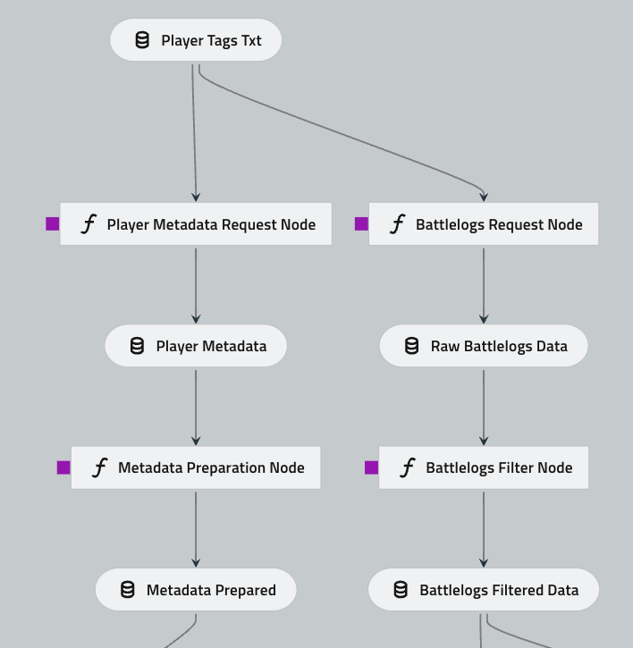
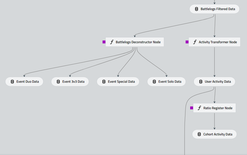
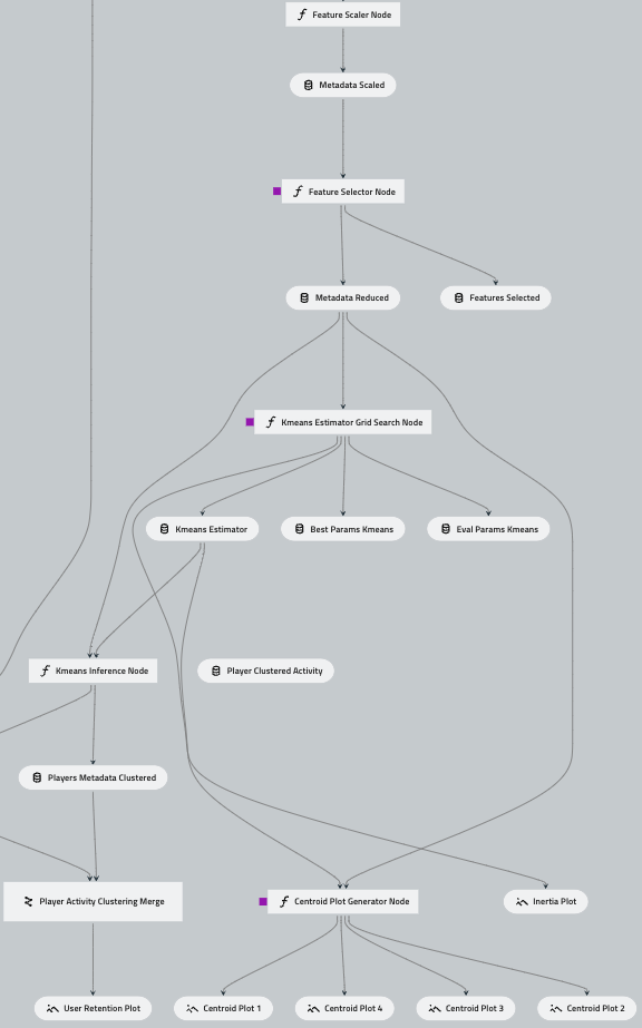
⚡Pipelines workflow

The pipeline architecture consists of five modular pipelines, with a total of 14 nodes. These pipelines will be constructed utilizing the open-source framework, Kedro.

Two of these pipelines, battlelogs_request_preprocess and metadata_request_preprocess, will use asynchronous coroutines to request data from the API and Spark for preprocessing. The requested data will be processed in batches of over 400 MB using only Spark to avoid communication overhead while minimizing the number of actions taken to take advantage of the worker’s process fluency.
The events_activity_segmentation pipeline will use Spark SQL API to produce retention metrics. This pipeline will use the data gathered from the requesting nodes. It is important to consider the data dependency between functions, which is why multithreading won’t be used.
Another pipeline, the player_cohorts_classifier, will perform a multiprocessing step over a Grid Search and cross-validation across multiple cores to evaluate the best quantity of clusters in which we can classify the players based on the game modes’ behaviors. This depends on the distortion rate and the hyperparameters defined by the user.
The last modular pipeline, player_activity_clustering_merge, will use the curated data to produce retention plots. It will use a single Python processing since it uses filtered data, which is a smaller subset.

This pipeline was designed to speed up processing by parallelizing. We can calculate the theoretical speedup by applying Amdahl’s Law.

$$S = \frac{1}{1-P+\frac{P}{N}} = \frac{1}{1-0.64286+\frac{0.64286}{10}} = 2.52$$

The theoretical speedup will be approximately 2.52 for a single-machine cluster. Here, S represents theoretical speedup, P represents the fraction of the workload that can be parallelized, and N represents the number of processors.

If you want to learn more about the appropriate use cases for multithreading and multiprocessing, I highly recommend watching this conference video by Chin Hwee Ong (Pycon Taiwan, 2020). It’s one of the best resources to get started.

⚔️ Battlelogs and Metadata Request Pipelines

Pipeline battlelogs_request_preprocess and metadata_request_preprocess

Both pipelines follow the same structure, the only difference is the request function used to gather the data from the API, one uses .get_battle_logs(), and the other uses the .get_player() function. And from these functions come two different data models battle logs and players.

Node: battlelogs_request_node and player_metadata_request_node

The inconsistent batch sizes of our data make it unsuitable to rely on an O(n) frequency expectation, due factors such as:

Product cycle (e.g., new feature or season launch).
Player longevity can affect the data (e.g., newer players with less than 25 sessions).

To extract the logs, I opted to use low-level APIs, specifically Python’s asynchronous coroutines. This approach allows executing one batch while waiting for a response from another, which is particularly helpful when dealing with variable batch sizes or waiting for processing, such as querying from a SQL database. However, the API wrapper used limits the multithreading pool size to 10, which means we had to separate the tags into batches of that size.

The main advantage of this approach is that it makes the code independent of the processor’s clock speed, avoiding waiting times between requests. Although Python’s Global Interpreter Lock (GIL) restricts running multiple threads simultaneously, we overcame this limitation by using coroutines to process future objects. If the pool size weren’t limited, we could have used multithreading instead. Overall, this strategy allowed us to process our data more efficiently and achieve better results.

  1
  2
  3
  4
  5
  6
  7
  8
  9
 10
 11
 12
 13
 14
 15
 16
 17
 18
 19
 20
 21
 22
 23
 24
 25
 26
 27
 28
 29
 30
 31
 32
 33
 34
 35
 36
 37
 38
 39
 40
 41
 42
 43
 44
 45
 46
 47
 48
 49
 50
 51
 52
 53
 54
 55
 56
 57
 58
 59
 60
 61
 62
 63
 64
 65
 66
 67
 68
 69
 70
 71
 72
 73
 74
 75
 76
 77
 78
 79
 80
 81
 82
 83
 84
 85
 86
 87
 88
 89
 90
 91
 92
 93
 94
 95
 96
 97
 98
 99
100
101
102
103
104
105
106
107
108
109
110
111
112
113
114
115
116
117
118
119
120
121


def battlelogs_request(
    player_tags_txt: str, parameters: Dict[str, Any]
) -> pd.DataFrame:
    """
    Extracts battlelogs from Brawlstars API by asynchronously executing a list of
    futures objects, each of which is made up of an Async thread task due to blocking
    call limitations of the api_request submodule.
    Args:
        player_tags_txt: A list of player tags.
        parameters: Additional parameters to be included in the API request.
    Returns:
         A structured DataFrame that concatenates all the battlelogs of the players.
    """
    # Get key and validate it exists
    API_KEY = conf_credentials.get("brawlstars_api", None).get("API_KEY", None)
    try:
        assert API_KEY is not None
    except AssertionError:
        log.info(
            "No API key has been defined. Request one at https://developer.brawlstars.com/"
        )

    # Create a BrawlStats client object to interact with the API. Note: the
    # "prevent_ratelimit" function in the source code can be used this behavior
    client = brawlstats.Client(token=API_KEY)

    # Split the player tags text by commas to create a list of player tags.
    player_tags_txt = player_tags_txt.split(",")

    def api_request(tag: str) -> pd.DataFrame:
        """Requests and structures the 25 most recent battle logs from the Brawl
        Stars API for a given player."""
        try:
            # Retrieve raw battle logs data from API
            player_battle_logs = client.get_battle_logs(tag).raw_data
            # Normalize data into structured format
            player_battle_logs_structured = pd.json_normalize(player_battle_logs)
            # Add player ID to DataFrame
            player_battle_logs_structured["player_id"] = tag
        except:
            log.info(f"No battle logs extracted for player {tag}")
            player_battle_logs_structured = pd.DataFrame()
            pass
        return player_battle_logs_structured

    async def api_request_async(tag: str) -> pd.DataFrame:
        """
        Transform non-sync request function to async coroutine, which creates
        a future object by API request.
        The Coroutine contains a blocking call that won't return a log until it's
        complete. So, to run concurrently, await the thread and not the coroutine by
        using this method.
        """
        return await asyncio.to_thread(api_request, tag)

    async def spawn_request(player_tags_txt: list) -> pd.DataFrame:
        """
        This asynchronous function takes a list of player tags as input and creates a
        list of coroutines that request the player's battlelogs data. It then
        schedules their execution and waits for them to complete by using the
        asyncio.gather() method. Finally, it concatenates all the dataframes returned by
        the coroutines into one dataframe.
        """
        start = time.time()
        log.info(f"Battlelogs request process started")
        # Create a list of coroutines and schedule their execution
        requests_tasks = [
            asyncio.create_task(api_request_async(tag)) for tag in player_tags_txt
        ]
        # Wait for all tasks to complete and gather their results
        battlelogs_data_list = await asyncio.gather(*requests_tasks)
        # Concatenate all the dataframes returned by the coroutines into one
        raw_battlelogs = pd.concat(battlelogs_data_list, ignore_index=True)
        log.info(
            f"Battlelogs request process finished in {time.time() - start} seconds"
        )
        return raw_battlelogs

    def activate_request(n: int = None) -> pd.DataFrame:
        """
        This function checks if a sampling limit is provided, and if so, it calls the
        spawn_request() function to request the battlelogs data of the first n
        players. If n is not provided, it splits the player tags list into batches of 10
        and calls the spawn_request() function for each batch. It then concatenates
        the dataframes returned by each call into one.
        """
        raw_battlelogs = pd.DataFrame()
        if n:
            # Call spawn_request() for the first n players
            raw_battlelogs = asyncio.run(spawn_request(player_tags_txt[:n]))
        else:
            # Split the tags list into batches of 10 and call spawn_request() for each
            split_tags = np.array_split(player_tags_txt, len(player_tags_txt) / 10)
            for batch in split_tags:
                raw_battlelogs_tmp = asyncio.run(spawn_request(batch))
                # Concatenate the dataframes returned by each call into one
                try:
                    raw_battlelogs = pd.concat(
                        [raw_battlelogs, raw_battlelogs_tmp], axis=0, ignore_index=True
                    )
                except:
                    pass

        return raw_battlelogs

    # Call activate_request() with the specified battlelogs_limit parameter
    raw_battlelogs = activate_request(n=parameters["battlelogs_limit"])

    # Replace dots in column names with underscores
    raw_battlelogs.columns = [
        col_name.replace(".", "_") for col_name in raw_battlelogs.columns
    ]

    # Check if the data request was successful
    try:
        assert not raw_battlelogs.empty
    except AssertionError:
        # Log an error message if no Battlelogs were extracted
        log.info("No Battlelogs were extracted. Please check your Client Connection")

    return raw_battlelogs

Here was collected a substantial amount of battle logs and player metadata, amounting to 476 MB and 453 MB, respectively. To analyze the process efficiency, was compared a synchronous process using a loop with an asynchronous process. The results were benchmarked:

The asynchronous process completed the task in just 287.93 seconds.
The synchronous process took 1004.54 seconds.

This translates to a 71% improvement in speed for the logs request, demonstrating the effectiveness of the new approach. Upon further analysis, out of the 23841 Player Tags, only 9104 had a battle log registry. Nevertheless, we managed to retrieve player metadata for 22738 of them, which is a good number considering we were using a public non-official API.

Node: battlelogs_filtering_node and metadata_preparation_node

  1
  2
  3
  4
  5
  6
  7
  8
  9
 10
 11
 12
 13
 14
 15
 16
 17
 18
 19
 20
 21
 22
 23
 24
 25
 26
 27
 28
 29
 30
 31
 32
 33
 34
 35
 36
 37
 38
 39
 40
 41
 42
 43
 44
 45
 46
 47
 48
 49
 50
 51
 52
 53
 54
 55
 56
 57
 58
 59
 60
 61
 62
 63
 64
 65
 66
 67
 68
 69
 70
 71
 72
 73
 74
 75
 76
 77
 78
 79
 80
 81
 82
 83
 84
 85
 86
 87
 88
 89
 90
 91
 92
 93
 94
 95
 96
 97
 98
 99
100
101
102
103
104


def battlelogs_filter(
    raw_battlelogs: pd.DataFrame, parameters: Dict
) -> pyspark.sql.DataFrame:
    """
    Filter players into cohorts (samples) for a predefined study using time ranges
    specified in the parameters. Also transforms datetime format from ISO 8601 to
    java.util.GregorianCalendar for Spark processing.
    Args:
        raw_battlelogs: Dataframe of concatenated battlelogs for all players
        parameters: Dictionary containing time ranges and DDL schema
    Returns:
        Filtered PySpark DataFrame containing only cohorts and necessary features
    """
    # Call | Create Spark Session
    spark = SparkSession.builder.getOrCreate()

    # Load and validate battlelogs data against the provided DDL schema
    try:
        battlelogs_filtered = spark.createDataFrame(
            data=raw_battlelogs, schema=parameters["raw_battlelogs_schema"][0]
        )
        # Convert lists stored as strings to Arrays of dictionaries
        battlelogs_filtered = battlelogs_filtered.withColumn(
            "battle_teams", f.from_json("battle_teams", t.ArrayType(t.StringType()))
        ).withColumn(
            "battle_players", f.from_json("battle_players", t.ArrayType(t.StringType()))
        )
    except TypeError:
        # If DDL schema for the battlelogs is incorrect, raise an error
        log.warning(
            "Type error on the DDL schema for the battlelogs,"
            'check "raw_battlelogs_schema" on the node parameters'
        )
        raise

    # Exclude missing events ids (519325->483860, not useful for activity aggregations)
    if parameters["exclude_missing_events"]:
        battlelogs_filtered = battlelogs_filtered.filter("event_id != 0")

    # Validate if a player is a battlestar player
    battlelogs_filtered = battlelogs_filtered.withColumn(
        "is_starPlayer",
        f.when(f.col("battle_starPlayer_tag") == f.col("player_id"), 1).otherwise(0),
    )

    # Filter the battlelogs data based on the specified timestamp range, and extract
    # a separate cohort to exclude specific dates if required
    if parameters["cohort_time_range"]:
        if "battleTime" not in battlelogs_filtered.columns:
            raise ValueError('Dataframe does not contain "battleTime" column.')
        else:
            # Convert timestamp strings to date format, where original timestamps are
            # in ~ ISO 8601 format (e.g. 20230204T161026.000Z)
            convertDT = f.udf(
                lambda string: dt.datetime.strptime(string, "%Y%m%dT%H%M%S.%fZ").date()
            )
            battlelogs_filtered = battlelogs_filtered.withColumn(
                "battleTime", convertDT("battleTime")
            )
            # Convert Java.util.GregorianCalendar date format to PySpark
            pattern = (
                r"(?:.*)YEAR=(\d+).+?MONTH=(\d+).+?DAY_OF_MONTH=(\d+)"
                r".+?HOUR=(\d+).+?MINUTE=(\d+).+?SECOND=(\d+).+"
            )
            battlelogs_filtered = battlelogs_filtered.withColumn(
                "battleTime",
                f.regexp_replace("battleTime", pattern, "$1-$2-$3 $4:$5:$6").cast(
                    "timestamp"
                ),
            ).withColumn("battleTime", f.date_format("battleTime", format="yyyy-MM-dd"))

        # Initialize an empty list to store DataFrames for each cohort
        cohort_selection = []
        # Assign an integer value to identify each sample cohort
        cohort_num = 1
        # Iterate over the cohort_time_range to subset the battlelogs_filtered DataFrame
        for date_range in parameters["cohort_time_range"]:
            # Filter the DataFrame based on the specified time range
            cohort_range = battlelogs_filtered.filter(
                (f.col("battleTime") > literal_eval(date_range)[0])
                & (f.col("battleTime") < literal_eval(date_range)[1])
            )
            # Add a new column to the DataFrame to identify the cohort it belongs to
            cohort_range = cohort_range.withColumn("cohort", f.lit(cohort_num))
            # Increment the cohort number for the next iteration
            cohort_num += 1
            # Append the cohort DataFrame to the cohort_selection list
            cohort_selection.append(cohort_range)
        # Concatenate all cohort DataFrames into one
        battlelogs_filtered = reduce(DataFrame.unionAll, cohort_selection)

    else:
        log.warning(
            "Please define at least one time range for your cohort. Check the "
            "parameters."
        )
        raise

    # Add a unique identifier column to the DataFrame
    battlelogs_filtered = battlelogs_filtered.withColumn(
        "battlelog_id", f.monotonically_increasing_id()
    )

    return battlelogs_filtered

The node serves two main purposes:

Transform retrieved data into a Spark data frame, ensuring accurate and consistent data with the expected data types.
Enable users to specify time ranges for player cohorts. This feature empowers users to customize the quantity and number of cohorts needed for their specific study.

For instance, in the following example, the cohorts are divided into 8 time-ranges. Events with missing identifiers are automatically excluded. This function assumes that the user requires a model capable of defining cohorts based on factors such as installation date or any other classification parameter.

 1
 2
 3
 4
 5
 6
 7
 8
 9
10
11
12
13
14
15
16
17
18
19
20
21
22
23
24
25
26
27
28
29
30


# ----- Parameters for preprocessing and filtering ----
battlelogs_filter:
  exclude_missing_events: true
  cohort_time_range:
    - ("2019-10-11","2020-04-10")
    - ("2020-04-11","2020-10-10")
    - ("2020-10-11","2021-04-10")
    - ("2021-04-11","2021-10-10")
    - ("2021-10-11","2022-04-10")
    - ("2022-04-11","2022-10-10")
    - ("2022-10-11","2023-04-10")
    - ("2023-04-11","2023-10-10")
  raw_battlelogs_schema:
    - "battleTime STRING, 
       event_id BIGINT, 
       event_mode STRING,
       event_map STRING,
       battle_mode STRING,
       battle_type STRING,
       battle_result STRING,
       battle_duration BIGINT,
       battle_trophyChange BIGINT,
       battle_starPlayer_tag STRING,
       battle_starPlayer_name STRING,
       battle_starPlayer_brawler_id BIGINT,
       battle_starPlayer_brawler_name STRING,
       battle_starPlayer_brawler_power BIGINT,
       battle_starPlayer_brawler_trophies BIGINT,
       battle_teams STRING,
       ... 

🕰️ Events and Activity Segmentation Pipeline

Pipeline events_activity_segmentation

Our goal is to transform raw data into valuable insights. To achieve this, we will focus on processing and filtering battle logs to produce “activity” data. This includes segmentations per event type, retention metrics, and ratios based on retention. With these metrics, we can gain a deeper understanding of user behavior and make informed decisions that drive growth.

Node: battlelogs_deconstructor_node

 1
 2
 3
 4
 5
 6
 7
 8
 9
10
11
12
13
14
15
16
17
18
19
20
21
22
23
24
25
26
27
28
29
30
31
32
33
34
35
36
37
38
39
40
41
42
43
44
45
46
47
48
49
50
51
52
53
54
55
56
57
58
59
60
61
62
63
64
65
66
67
68
69
70
71
72
73
74
75
76
77
78
79
80
81


def battlelogs_deconstructor(
    battlelogs_filtered: pyspark.sql.DataFrame, parameters: Dict[str, Any]
) -> Tuple[
    pyspark.sql.DataFrame,
    pyspark.sql.DataFrame,
    pyspark.sql.DataFrame,
    pyspark.sql.DataFrame,
]:
    """
    Extract player and brawler combinations from the same team or opponents,
    grouped in JSON format, based on user-defined event types.
    Each of the 'exploders' is parameterized by the user, according to the number of
    players needed for each type of event.
    Args:
        battlelogs_filtered: a filtered Pyspark DataFrame containing relevant cohorts
        and features.
        parameters: a dictionary of event types defined by the user to include in the
        subset process.
    Returns:
        A tuple of four Pyspark DataFrames, each containing only one event type
    """
    # Call | Create Spark Session
    spark = SparkSession.builder.getOrCreate()

    log.info("Deconstructing Solo Events")
    if parameters["event_solo"] and isinstance(parameters["event_solo"], list):
        event_solo_data = battlelogs_filtered.filter(
            f.col("event_mode").isin(parameters["event_solo"])
        )
        event_solo_data = _group_exploder_solo(
            event_solo_data, parameters["standard_columns"]
        )
    else:
        log.warning(
            "Solo Event modes not defined or not found according to parameter list"
        )
        event_solo_data = spark.createDataFrame([], schema=t.StructType([]))

    log.info("Deconstructing Duo Events")
    if parameters["event_duo"] and isinstance(parameters["event_duo"], list):
        event_duo_data = battlelogs_filtered.filter(
            f.col("event_mode").isin(parameters["event_duo"])
        )
        event_duo_data = _group_exploder_duo(
            event_duo_data, parameters["standard_columns"]
        )
    else:
        log.warning(
            "Duo Event modes not defined or not found according to parameter list"
        )
        event_duo_data = spark.createDataFrame([], schema=t.StructType([]))

    log.info("Deconstructing 3 vs 3 Events")
    if parameters["event_3v3"] and isinstance(parameters["event_3v3"], list):
        event_3v3_data = battlelogs_filtered.filter(
            f.col("event_mode").isin(parameters["event_3v3"])
        )
        event_3v3_data = _group_exploder_3v3(
            event_3v3_data, parameters["standard_columns"]
        )
    else:
        log.warning(
            "3 vs 3 Event modes not defined or not found according to parameter list"
        )
        event_3v3_data = spark.createDataFrame([], schema=t.StructType([]))

    log.info("Deconstructing Special Events")
    if parameters["event_special"] and isinstance(parameters["event_special"], list):
        event_special_data = battlelogs_filtered.filter(
            f.col("event_mode").isin(parameters["event_special"])
        )
        event_special_data = _group_exploder_special(
            event_special_data, parameters["standard_columns"]
        )
    else:
        log.warning(
            "Special Event modes not defined or not found according to parameter list"
        )
        event_special_data = spark.createDataFrame([], schema=t.StructType([]))

    return event_solo_data, event_duo_data, event_3v3_data, event_special_data

To understand the basic game modes of this mobile game, an extensive research was required. All assumptions made in the event deconstruction process are based on the information provided by the Brawl Stars Fandom Wiki.

The deconstruction process will classify the battle_teams column and divide all players in each session into groups based on the number of team members defined by the event type. These event types are categorized according to specific parameters, enabling users to easily classify events based on the distribution of players' teams per session.

 1
 2
 3
 4
 5
 6
 7
 8
 9
10
11
12
13
14
15
16
17
18
19
20
21


# ----- Parameters to deconstruct the data by event ----
battlelogs_deconstructor:
  event_solo: ['soloShowdown']
  event_duo: ['duoShowdown']
  event_3v3: ['gemGrab','brawlBall','bounty','heist','hotZone','knockout']
  event_special: ['roboRumble','bossFight','lastStand', 'bigGame']
  standard_columns:
    - 'battlelog_id'
    - 'cohort'
    - 'battleTime'
    - 'player_id'
    - 'event_id'
    - 'event_mode'
    - 'event_map'
    - 'is_starPlayer'
    - 'battle_type'
    - 'battle_result'
    - 'battle_rank'
    - 'battle_duration'
    - 'battle_trophyChange'
    - 'battle_level_name'

The use of parameters to segment the raw battle logs data is interpreted as follows:

The battle_teams column in the JSON files contains a massive collection of data. When the battle type is in the list ['gemGrab','brawlBall','bounty','heist','hotZone','knockout'], the code recognizes this as 3 vs 3 events, meaning that the battle teams column contains information on all six players.

To create the players_collection and brawlers_collection data, the six players are divided into two groups. This division results in two collections that provide valuable insights into player behavior and brawler selection.

1
2
3


players_collection >> [[#2882QV9J0, #28Y9GJC0L, #2UPL0QCYG], [#U08LRGYJ, #2QQ9GY2YL, #22UJ88YQ9]]

brawlers_collection >> [[CROW, MORTIS, BUZZ], [MORTIS, SURGE, DYNAMIKE]]

By conducting an interaction study between players and the brawlers or characters they use, a data scientist can extract valuable insights into gameplay. For instance, if you’re curious about how the exploder function works, you’ll find this code particularly useful. Its high density is evidence of Spark high performance, which has enabled the minimization of Spark actions performed. However, you can satisfy your curiosity here.

Node: activity_transformer_node

  1
  2
  3
  4
  5
  6
  7
  8
  9
 10
 11
 12
 13
 14
 15
 16
 17
 18
 19
 20
 21
 22
 23
 24
 25
 26
 27
 28
 29
 30
 31
 32
 33
 34
 35
 36
 37
 38
 39
 40
 41
 42
 43
 44
 45
 46
 47
 48
 49
 50
 51
 52
 53
 54
 55
 56
 57
 58
 59
 60
 61
 62
 63
 64
 65
 66
 67
 68
 69
 70
 71
 72
 73
 74
 75
 76
 77
 78
 79
 80
 81
 82
 83
 84
 85
 86
 87
 88
 89
 90
 91
 92
 93
 94
 95
 96
 97
 98
 99
100
101
102
103
104
105
106
107
108
109
110
111
112
113
114
115
116
117
118
119
120
121
122


def activity_transformer(
    battlelogs_filtered: pyspark.sql.DataFrame, parameters: Dict[str, Any]
) -> pyspark.sql.DataFrame:
    """
    Converts filtered battlelogs activity into a wrapped format data frame,
    with retention metrics and n-sessions at the player level of granularity. It
    takes a set of parameters to extract the retention and number of sessions based
    on a 'cohort frequency' parameter.
    Args:
        battlelogs_filtered: Filtered Pyspark DataFrame containing only cohorts and
        features required for the study.
        parameters: Frequency of the cohort and days to extract for the output.
    Returns:
        Pyspark dataframe with retention metrics and n-sessions at the player level
        of granularity.
    Notes (parameters):
    - When 'daily' granularity is selected, the cohort period is the day of the
    user's  first event.
    - When 'weekly' granularity is selected, the cohort period is the first
    consecutive Monday on or after the day of the user's first event.
    - When 'monthly' granularity is selected, the cohort period is the first day of
    the month in which the user's first event occurred.
    Notes (performance):
    - The Cohort frequency transformation skips exhaustive intermediate transformations,
    such as 'Sort', since the user can insert many cohorts as they occur in the
    preprocessing stage, causing excessive partitioning.
    """
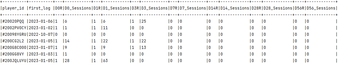
    # Aggregate user activity data to get daily number of sessions
    user_activity = (
        battlelogs_filtered.select("cohort", "battleTime", "player_id")
        .groupBy("cohort", "battleTime", "player_id")
        .count()
        .withColumnRenamed("count", "daily_sessions")
    )

    # Validate | Redefine Cohort Frequency, default to 'daily'
    time_freq, user_activity = _convert_user_activity_frequency(
        cohort_frequency=parameters["cohort_frequency"], user_activity=user_activity
    )

    # Create a window by each one of the player's window
    player_window = Window.partitionBy(["player_id"])

    # Find the first logged date per player in the cohort
    user_activity = user_activity.withColumn(
        "first_log", f.min(time_freq).over(player_window)
    )

    # Find days passed to see player return
    user_activity = user_activity.withColumn(
        "days_to_return", f.datediff(time_freq, "first_log")
    )

    # Subset columns and add counter variable to aggregate number of player further
    user_activity = user_activity.select(
        "cohort", "player_id", "first_log", "days_to_return", "daily_sessions"
    ).withColumn("player_count", f.lit(1))

    # List cohorts, iterate over them and append them to the final output
    cohort_list = [
        row.cohort for row in user_activity.select("cohort").distinct().collect()
    ]
    output_range = []

    for cohort in cohort_list:
        # Filter only data of the cohort in process
        tmp_user_activity = user_activity.filter(f.col("cohort") == cohort)

        # Pivot data from long format to wide
        tmp_user_activity = (
            tmp_user_activity.groupBy(["player_id", "first_log"])
            .pivot("days_to_return")
            .agg(
                f.sum("player_count").alias("day"),
                f.sum("daily_sessions").alias("day_sessions"),
            )
        )

        # Extract daily activity columns, save as arrays of column objects
        day_cohort_col = tmp_user_activity.select(
            tmp_user_activity.colRegex("`.+_day$`")
        ).columns
        day_cohort_col = f.array(*map(f.col, day_cohort_col))

        # Extract daily sessions counter columns, save as arrays of column objects
        day_sessions_col = tmp_user_activity.select(
            tmp_user_activity.colRegex("`.+_day_sessions$`")
        ).columns
        day_sessions_col = f.array(*map(f.col, day_sessions_col))

        # Empty list to allocate final columns
        cols_retention = []

        # Produce retention metrics and session counters
        for day in parameters["retention_days"]:
            # Define column names
            DDR = f"D{day}R"
            DDTS = f"D{day}_Sessions"
            # Obtain retention for a given day
            tmp_user_activity = tmp_user_activity.withColumn(
                DDR, retention_metric(day_cohort_col, f.lit(day))
            )
            # Obtain total of sessions until given day
            tmp_user_activity = tmp_user_activity.withColumn(
                DDTS, sessions_sum(day_sessions_col, f.lit(day))
            ).withColumn(DDTS, f.when(f.col(DDR) != 1, 0).otherwise(f.col(DDTS)))
            # Append final columns
            cols_retention.append(DDR)
            cols_retention.append(DDTS)

        # Final formatting
        standard_columns = ["player_id", "first_log"]
        standard_columns.extend(cols_retention)
        tmp_user_activity = tmp_user_activity.select(*standard_columns)

        # Append cohort's user activity data to final list
        output_range.append(tmp_user_activity)

    # Reduce all dataframe to overwrite original
    user_activity_data = reduce(DataFrame.unionAll, output_range)

    return user_activity_data

Imagine having the capacity to transform filtered battle logs activity into a wrapped format data frame that delivers retention metrics and n-sessions at the player level of granularity. That’s exactly what this node does. Using a set of customizable parameters, it extracts the retention and number of sessions based on a cohort frequency parameter:

When you select daily granularity, the cohort period is based on the day of the user’s first event, showing you the number of sessions logged per user on the day they installed the game, on the day they returned, and so on.
If you choose weekly granularity, the cohort period is based on the first consecutive Monday on or after the day of the user’s first event. This allows you to track user behavior on a weekly basis, providing valuable insights into how engagement fluctuates throughout the week.
And if you opt for monthly granularity, the cohort period is based on the first day of the month in which the user’s first event occurred. This gives you an overview of user behavior on a monthly basis, perfect for understanding trends over time.

By default, this node is set to daily, making it easy to get started and quickly visualize your data. With its intuitive and powerful features, you’ll gain deeper insights into your users' behavior, and be able to optimize your game for even greater success.

Each one of the days to measure can be defined as parameters as well, to let the user define the criteria of the retention study:

 1
 2
 3
 4
 5
 6
 7
 8
 9
10
11


# ----- Parameters to extract activity day per user ----
activity_transformer:
  cohort_frequency: daily
  retention_days:
    - 0
    - 1
    - 3
    - 7
    - 14
    - 28
    - 56

Node: ratio_register_node

 1
 2
 3
 4
 5
 6
 7
 8
 9
10
11
12
13
14
15
16
17
18
19
20
21
22
23
24
25
26
27
28
29
30
31
32
33
34
35
36
37
38
39
40
41
42
43
44
45
46
47
48
49
50
51
52
53
54
55
56
57
58
59
60
61
62
63
64
65
66
67
68


def ratio_register(
    user_activity: pyspark.sql.DataFrame,
    params_rat_reg: Dict[str, Any],
    params_act_tran: Dict[str, Any],
) -> pyspark.sql.DataFrame:
    """
    Takes Activity per Day from the "activity_transformer_node" (E.G: columns DXR),
    builds retention ratios per day using a bounded retention calculation.
    Args:
        user_activity: Pyspark dataframe with retention metrics and n-sessions at the
        player level of granularity.
        params_rat_reg: Parameters to aggregate retention metrics, based on User inputs.
        params_act_tran: Parameters to extract activity day per user, based on User.
        inputs.
    Returns:
        Pyspark dataframe with bounded retention ratios aggregated.
    """
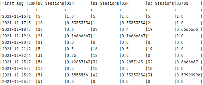
    # Request parameters to validate
    days_available = params_act_tran["retention_days"]
    ratios = [literal_eval(ratio) for ratio in params_rat_reg["ratios"]]

    # Validate day labels are present in parameters
    _ratio_days_availabilty(ratios, days_available)

    # Grouping + renaming multiple columns: https://stackoverflow.com/a/74881697
    retention_columns = [
        col for col in user_activity.columns if col not in ["player_id", "first_log"]
    ]
    aggs = [f.expr(f"sum({col}) as {col}") for col in retention_columns]
    # Apply aggregation
    cohort_activity_data = user_activity.groupBy("first_log").agg(*aggs)

    # Obtain basics retention ratios aggregated
    for ratio in ratios:
        num, den = ratio
        ratio_name = f"D{num}R"
        ret_num = f"D{num}R"
        ret_den = f"D{den}R"
        cohort_activity_data = cohort_activity_data.withColumn(
            ratio_name, ratio_agg(f.col(ret_num), f.col(ret_den))
        )

    # Obtain analytical ratios if them were defined in the parameters (ratio register)
    if params_rat_reg["analytical_ratios"] and isinstance(
        params_rat_reg["analytical_ratios"], list
    ):
        # Request parameters to validate
        analytical_ratios = [
            literal_eval(ratio) for ratio in params_rat_reg["analytical_ratios"]
        ]
        # Validate day labels are present in parameters
        _ratio_days_availabilty(analytical_ratios, days_available)
        # Obtain basics retention ratios aggregated
        for ratio in analytical_ratios:
            num, den = ratio
            ratio_name = f"D{num}/D{den}"
            ret_num = f"D{num}R"
            ret_den = f"D{den}R"
            cohort_activity_data = cohort_activity_data.withColumn(
                ratio_name, ratio_agg(f.col(ret_num), f.col(ret_den))
            )
    else:
        log.info("No analytical ratios were defined")

    # Reorganization per log date
    cohort_activity_data = cohort_activity_data.orderBy(["first_log"])

    return cohort_activity_data

In the final stage of this pipeline, we’ll generate bounded retention metrics as ratios. These metrics will be used to demonstrate the effectiveness of our approach. While I may not have experience in gaming, I understand the importance of accurately measuring retention ratios. To ensure our metrics are properly measured, we’ll ask the Andreessen Horowitz Partner, Andrew Chen, a leading expert in the field.

6) D1/D7/D30 that exceeds 60/30/15 (daily frequency)
7) revenue or activity expansion on a *per user* basis over time -- indicates deeper engagement / habit formation
8) >60% organic acquisition -- CAC doesn't even matter!

Having even one is impressive -- it'd make me sit up!
— andrew chen (@andrewchen) October 15, 2019

Well, the consultation went smoothly. So, we’re ready to define our parameters. Specifically, we’ll be establishing ratios for individual retention metrics, as well as ratios for combined retention metrics (analytical ratios):

 1
 2
 3
 4
 5
 6
 7
 8
 9
10
11
12
13


# ----- Parameters to aggregate retention metrics ----
ratio_register:
  ratios:
    - (1,0)
    - (3,0)
    - (7,0)
    - (14,0)
    - (28,0)
    - (56,0)
  analytical_ratios:
    - (3,1) # D3/D1
    - (7,3) # D7/D3
    - (28,7) # D28/D7

To gain a deeper understanding of retention metrics, I highly recommend delving into Timothy Daniel’s (2022) insightful article.

In essence, there are two types of retention metrics: bounded and unbounded. While the latter includes unique users returning on the same day or later, the first one is considered more reliable because it’s not influenced by new data coming in. So if we’re aiming for accuracy and consistency in the retention measurements, bounded retention should be the go-to.

This is how the output should look like:

💀 Player Classification and Cohorts Creation Pipeline

Pipeline player_cohorts_classifier

This pipeline is a parametrized method for classifying players. It saves the model in the registry and the artifacts for each experiment. The main objective of this pipeline is to make it easy for data scientists to set hyperparameters and save their models. This will help to prevent the spread of models across a repository into random Jupyter notebooks, without versioning. We know this is a common scenario that many data scientists are familiar with.

It is worth mentioning that each node in this pipeline was planned using an experimental Jupyter Notebook. If you want to check the raw version, you can download it from here.

Node: feature_scaler_node

 1
 2
 3
 4
 5
 6
 7
 8
 9
10
11
12
13
14
15
16
17
18
19
20
21
22
23
24
25
26
27
28
29
30
31
32


def feature_scaler(metadata_prepared: pd.DataFrame) -> pd.DataFrame:
    """
    Applies MaxAbsScaler on the input data and returns the transformed data.
    Args:
        metadata_prepared: Dataframe containing player metadata with 'player_id'
        column and numeric features.
    Returns:
        Dataframe with scaled numeric features
    Raises:
        AssertionError: If the length of 'player_id' column and the transformed data are
        not equal
    """
    # Drop the 'player_id' column and use it as the target variable
    X = metadata_prepared.drop("player_id", axis=1)
    y = metadata_prepared["player_id"]

    # Initialize the MaxAbsScaler object, fit it to the data, and transform the data
    scaler = MaxAbsScaler()
    X_scaled = scaler.fit_transform(X)

    # Create a new DataFrame with the transformed data and original column names
    metadata_scaled = pd.DataFrame(X_scaled, columns=X.columns)

    # Check if the length of 'y' matches the transformed data and concatenate them
    try:
        assert len(y) == len(metadata_scaled)
        metadata_scaled = pd.concat([y, metadata_scaled], axis=1)
    except AssertionError:
        log.info("Scaler instance or data is corrupted, try debugging your input data")

    # Return the scaled DataFrame
    return metadata_scaled

This node will use as input the player metadata, which includes descriptive data about the lifetime statistics for each player per battle-type score, to get more detail on the data specs you can refer to the “Player” data model.

To train a KMeans model effectively, it’s crucial to prepare the data by scaling it. Let’s first review one of my recent experiments before delving into the scaling methods. The scaling method we choose depends on the nature of the data and our analysis requirements. To choose the best scaling method for your project, here’s a brief overview of each option:

StandardScaler: This scaling method scales each feature to have a mean of 0 and a standard deviation of 1. It’s a good choice if our data follow a normal distribution and if we want to emphasize the differences between data points.
Normalizer: This scaling method scales each sample to have a Euclidean length of 1. It’s a good choice if we want to emphasize the direction of the data points and we’re not interested in their magnitude.
MaxAbsScaler: This scaling method scales each feature to have a maximum absolute value of 1. It’s a good choice if we have sparse data or features with very different scales and we want to preserve the sparsity and relative magnitudes of the data, like when we have justified outliers.

So, as we have sparse data and features with very different scales, and we want to preserve the sparsity and relative magnitudes of the data I used MaxAbsScaler.

Node: feature_selector_node

 1
 2
 3
 4
 5
 6
 7
 8
 9
10
11
12
13
14
15
16
17
18
19
20
21
22
23
24
25
26
27
28
29
30
31
32
33
34
35
36
37
38
39
40
41
42
43
44


def feature_selector(
    metadata_scaled: pd.DataFrame, parameters: Dict[str, Any]
) -> Tuple[pd.DataFrame, Dict[str, List]]:
    """
    Select top K features from a scaled metadata dataframe. Here the module select
    n_features_to_select to consider the selection of features to represent:
        - Player capacity of earning credits (representation of trophies).
        - Capacity of being a team player (representation of 3v3 or Duo victories).
        - Solo skills (representation of Solo victories).
    Args:
        metadata_scaled: The input metadata as a Pandas DataFrame, with player ID in
        one column and feature values in the remaining columns.
        parameters: A dictionary of input parameters, containing the number of top
        features to select.
    Returns:
        A new metadata dataframe containing only the selected top K features,
        with the same player ID column as the input dataframe
    """
    # Drop the player ID column from the metadata dataframe
    X_scaled = metadata_scaled.drop("player_id", axis=1)
    # Extract the player ID column from the metadata dataframe
    y = metadata_scaled["player_id"]

    # Use SelectKBest and ColumnTransformer to select the top K features
    selector = SelectKBest(f_classif, k=parameters["top_features"])
    preprocessor = ColumnTransformer(
        transformers=[("SKB_transformer", selector, X_scaled.columns)]
    )
    preprocessor.fit(X_scaled, y)
    # Extract the feature-selected data from the preprocessor object
    X_features = preprocessor.transform(X_scaled)

    # Get the index numbers and names of the selected columns
    new_columns_index = preprocessor.named_transformers_["SKB_transformer"].get_support(
        indices=True
    )
    new_columns_names = X_scaled.columns[new_columns_index]
    log.info(f"Columns selected: {new_columns_names}")

    # Create a new dataframe with only the selected columns
    X_features = pd.DataFrame(X_features, columns=new_columns_names)
    metadata_reduced = pd.concat([y, X_features], axis=1)

    return metadata_reduced, {"features_selected": list(new_columns_names)}

To ensure a correct classification process, it is important to select appropriate features to classify players, but it is equally important to determine the appropriate way to do so. In this case, I did not use a scientific approach to define it, but rather based it on game criteria.

I considered four attributes based on the next metrics:

Trophies: The number of trophies earned by a player in Brawlstars is a significant indicator of their performance level and skill.
3 vs. 3 Victories: This attribute shows how many 3 vs. 3 matches the player has won, which could be an indication of their teamwork ability.
Solo and Duo Victories: These attributes represent the number of Solo or Duo matches the player has won, indicating their ability to play effectively without the support of teammates.
Best RoboRumbleTime: This attribute represents the player’s best time in defeating robots in the Robo Rumble event, indicating their skill in handling PvE (player versus environment) situations.

Note: Since highestPowerPlayPoints refers to the highest score in a competitive mode that is no longer active, we will remove this feature. After all, according to Brawlstars Wiki, this competitive mode could be unlocked after earning a Star Power for any Brawler, meaning that won’t be a descriptive attribute for every player.

Also, these attributes can be divided into four descriptive inter-player interaction buckets: 3 vs. 3 Victories sessions, Duo and Solo sessions, and Experience. However, we will exclude PvE from this project since we should use different game design methods to ensure better analysis of the player’s behavior versus the environment.

To determine the most appropriate method to use, we need to select the variables that can give us better performance given a model construction. We have three options to consider:

VarianceThreshold: This method removes all features whose variance doesn’t meet a certain threshold. This technique is useful when our dataset has many features with low variance and can be removed without affecting the model’s performance.
SelectKBest: This technique selects the K most significant features based on statistical tests such as chi-squared or ANOVA.
Recursive Feature Elimination: This method recursively removes features and evaluates the model’s performance until the optimal number of features is reached. This method uses a model to assess the feature’s importance and removes the least important ones iteratively.

In conclusion, we also need to consider classifying players based on their preferred type of event and their historical score achieved, which is measured by trophies. We can group highly skilled players with good teamwork into a cluster, while players with high solo and duo victories can be classified as excellent solo and duo players.

By defining these clusters, we can gain insights into the behavior and tendencies of different types of players and develop more targeted game design strategies. Therefore, we will set the parameter k of the SelectKBest method as 4 to select the top 4 features that can give the best model performance on the scaled data, which are going to be saved and versioned in the /07_feature_store.

1
2
3


# ----- Parameters for feature selector ----
feature_selector:
  top_features: 4

Node: kmeans_estimator_grid_search_node

 1
 2
 3
 4
 5
 6
 7
 8
 9
10
11
12
13
14
15
16
17
18
19
20
21
22
23
24
25
26
27
28
29
30
31
32
33
34
35
36
37
38
39
40
41
42
43
44
45
46
47
48
49
50
51
52
53
54
55
56
57
58
59
60
61
62


def kmeans_estimator_grid_search(
    metadata_reduced: pd.DataFrame, parameters: Dict[str, Any]
) -> Tuple[Union[bytes, None], Dict[str, Any], Dict[str, Any], go.Figure]:
    """
    Perform a grid search with cross-validation to find the best hyperparameters for
    KMeans clustering algorithm.
    Args:
        metadata_reduced: The metadata of players to be clustered.
        parameters: The parameters for the grid search of the estimator.
    Returns:
        kmeans_estimator: Pickle file containing the KMeans estimator
        best_params_KMeans: The best parameters found by GridSearchCV
        eval_params_KMeans: The parameters evaluated by GridSearchCV
        inertia_plot: Inertia plot for a clustering grid search
    """
    # Drop the 'player_id' column from the 'metadata_reduced' dataframe
    X_features = metadata_reduced.drop(columns=["player_id"])

    # Define hyperparameters for KMeans algorithm
    seed = parameters.get("random_state")
    max_n_cluster = parameters.get("max_n_cluster")
    starting_point_method = parameters.get("starting_point_method", "random")
    max_iter = parameters.get("max_iter")
    distortion_tol = parameters.get("distortion_tol")
    cv = parameters.get("cross_validations")
    plot_dimensions = parameters.get("plot_dimensions")

    # Set hyperparameters for GridSearchCV
    eval_params_KMeans = {
        "n_clusters": range(2, max_n_cluster),
        "init": starting_point_method,
        "max_iter": max_iter,
        "tol": distortion_tol,
    }

    # Set number of CPUs to use
    cores = parameters.get("cores", -1)

    # Perform GridSearch Cross-Validation for KMeans instance
    log.info(
        f"Performing GridSearch Cross-Validation for KMeans instance\n"
        f"** Parameters in use **: {eval_params_KMeans}"
    )
    grid_search = GridSearchCV(
        KMeans(random_state=seed), param_grid=eval_params_KMeans, cv=cv, n_jobs=cores
    )
    grid_search.fit(X_features)

    # Extract best estimator
    kmeans_estimator = grid_search.best_estimator_

    # Retrieve parameters used to define the best estimator
    best_params_KMeans, eval_params_KMeans = _estimator_param_export(
        eval_params_KMeans, grid_search, seed
    )

    # Return inertia plot to visualize the best estimator
    inertia_plot = _inertia_plot_gen(
        grid_search, plot_dimensions, starting_point_method
    )

    return kmeans_estimator, best_params_KMeans, eval_params_KMeans, inertia_plot

We begin by obtaining the scaled data along with the selected features. Once the preparation is complete, we can proceed to train a model and create the estimator object. The resulting artifacts will be stored in our model registry, which can be found at the path /08_model_registry within our GCP bucket.

To determine the most suitable algorithm for our task, two key factors were considered: the dataset size and the desired number of clusters. For larger datasets, we favor the computationally efficient and faster K-Means algorithm. On the other hand, when working with smaller datasets, Hierarchical clustering emerges as a more appropriate choice.

K-Means is a highly effective partition-based clustering algorithm that groups data points into a predetermined number of clusters. It begins by randomly selecting initial centroids (cluster centers) and proceeds to iteratively assign each data point to the nearest centroid based on a chosen distance metric. After the assignment, the centroids are updated by calculating the mean distance of all the points within each cluster. This process repeats until the centroids no longer change, ensuring the clusters reach a stable state.

In summary, this particular node performs a grid search combined with cross-validation to identify the optimal hyperparameters for the KMeans clustering algorithm.

 1
 2
 3
 4
 5
 6
 7
 8
 9
10
11
12
13


# ----- Parameters for player clustering ----
kmeans_estimator_grid_search:
  random_state: 42
  max_n_cluster: 13
  starting_point_method: ["k-means++"]
  max_iter: [200]
  distortion_tol: [0.0001]
  cross_validations: 5
  cores: -1
  # Inertia plot dimensions in px
  plot_dimensions:
    width: 500
    height: 500

To enhance the evaluation process, we utilize the GridSearch method, allowing users to define and evaluate multiple parameters. Let’s explore the key parameters:

starting_point_method: This parameter determines the method for selecting initial centroids in the K-means algorithm. We employ the k-means++ initialization method, which enhances convergence by intelligently choosing initial centroids.
max_iter: The maximum number of iterations that the K-means algorithm will perform is specified by this parameter. The algorithm will halt either when it reaches the specified max_iter iterations or when convergence is achieved before that.
distortion_tol: This parameter controls the convergence criteria based on distortion (or inertia). The algorithm terminates if the change in distortion between two consecutive iterations falls below this value.
cores: Used to define the number of cores used by the machine to evaluate and select the best model.

By leveraging GridSearch, we can identify the model with the highest negative inertia. The selected model will be stored in the model registry as a pickle file. Additionally, a versioned inertia plot will be generated, enabling easy tracking of the number of clusters selected and evaluated.

The node will capture four outputs, each one versioned with the execution timestamp from the pipeline:

kmeans_estimator: This output stores the trained model as a pickle file.
best_params_KMeans: This output represents the optimal estimator chosen through the GridSearch method.
eval_params_KMeans: This output contains the hyperparameters used for evaluating the GridSearch.
inertia_plot: This output encompasses the inertia plot displayed earlier in the form of a Plotly JSON dataset.

Node: kmeans_inference_node

 1
 2
 3
 4
 5
 6
 7
 8
 9
10
11
12
13
14
15
16
17
18
19
20
21
22
23
24
25
26
27
28
29
30
31
32
33
34
35
36
37
38
39
40
41
42
43
44
45
46
47
48
49
50
51
52
53
54
55
56


def kmeans_inference(
    metadata_reduced: pd.DataFrame, kmeans_estimator: Union[bytes, None]
) -> Tuple[pd.DataFrame, Dict[str, Any]]:
    """
    Cluster players' metadata using K-Means algorithm and compute clustering
    evaluation metrics.
    The following clustering evaluation metrics are computed and logged:
        - Total Inertia Score
        - Silhouette Score
        - Davies-Bouldin Score
        - Calinski-Harabasz Score
    Args:
        metadata_reduced: DataFrame containing players' metadata to cluster.
        kmeans_estimator: Trained K-Means estimator (model).
    Returns:
        Clustered players' metadata and their corresponding cluster labels and a
        dictionary (metrics_KMeans) containing clustering evaluation metrics computed
    """
    # Drop the 'player_id' column from the 'metadata_reduced' dataframe
    X_features = metadata_reduced.drop(columns=["player_id"])

    # Extract the 'player_id' column from the 'metadata_reduced' dataframe
    y = metadata_reduced["player_id"]

    # Generate and append labels
    predicted_labels = kmeans_estimator.predict(X_features)
    player_metadata_clustered = pd.concat(
        [y, pd.Series(predicted_labels, name="cluster_labels"), X_features], axis=1
    )

    # Extract total inertia score
    inertia_score = kmeans_estimator.inertia_
    log.info(f"Total Inertia Score: {inertia_score:.2f}")

    # Extract Silhouette score
    silhouette = silhouette_score(X_features, predicted_labels)
    log.info(f"Silhouette Score: {silhouette:.2f}")

    # Extract Davies-Bouldin index
    davies_bouldin = davies_bouldin_score(X_features, predicted_labels)
    log.info(f"Davies-Bouldin Score: {davies_bouldin:.2f}")

    # Extract Calinski-Harabasz index
    calinski_harabasz = calinski_harabasz_score(X_features, predicted_labels)
    log.info(f"Calinski-Harabasz Score: {calinski_harabasz:.2f}")

    # Save metrics for tracking
    metrics_KMeans = {
        "silhouette_score": silhouette,
        "davies_bouldin_score": davies_bouldin,
        "calinski_harabasz_score": calinski_harabasz,
        "total_inertia": inertia_score,
    }
    metrics_KMeans = {str(key): value for key, value in metrics_KMeans.items()}

    return player_metadata_clustered, metrics_KMeans

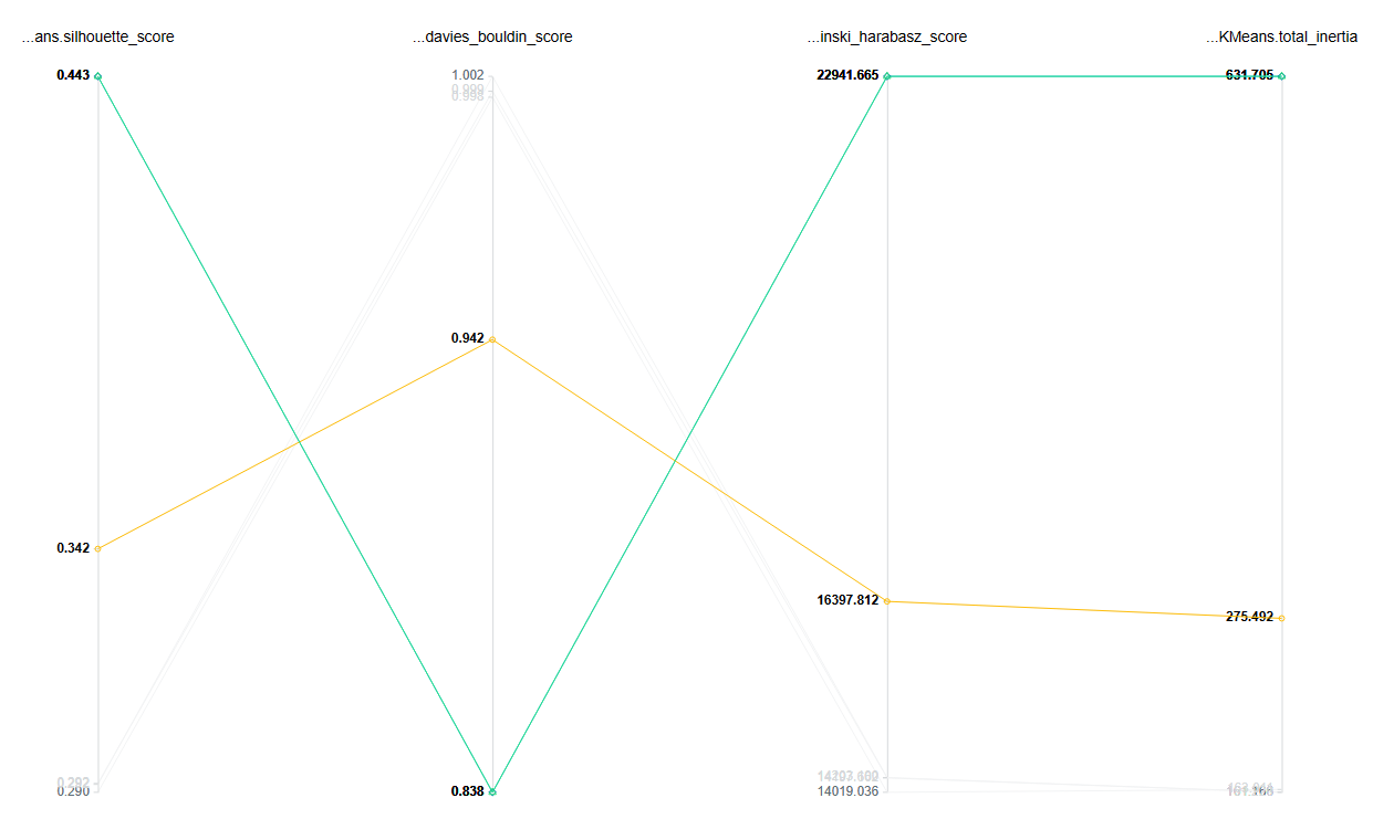
The next step is to evaluate the model. This node will import the model from the model registry, produce the inferences, and generate labels that will be saved in the player_metadata_clustered dataset. It will also produce four metrics to evaluate the model:

Inertia: This metric measures the sum of distances between each point and its assigned cluster center. A lower inertia value indicates that the data points are closer to their respective centroids.
Silhouette score: This metric indicates how well each data point is assigned to its cluster. A higher silhouette score indicates that data points within a cluster are more similar to each other and dissimilar to points in other clusters.
Davies-Bouldin index: This metric evaluates the average similarity between each cluster and its most similar cluster, taking into account both the scatter within the cluster and the separation between different clusters. A lower Davies-Bouldin index indicates a better separation between clusters.
Calinski-Harabasz index: This metric measures the ratio of between-cluster variance to within-cluster variance. A higher Calinski-Harabasz index indicates a better separation between clusters.

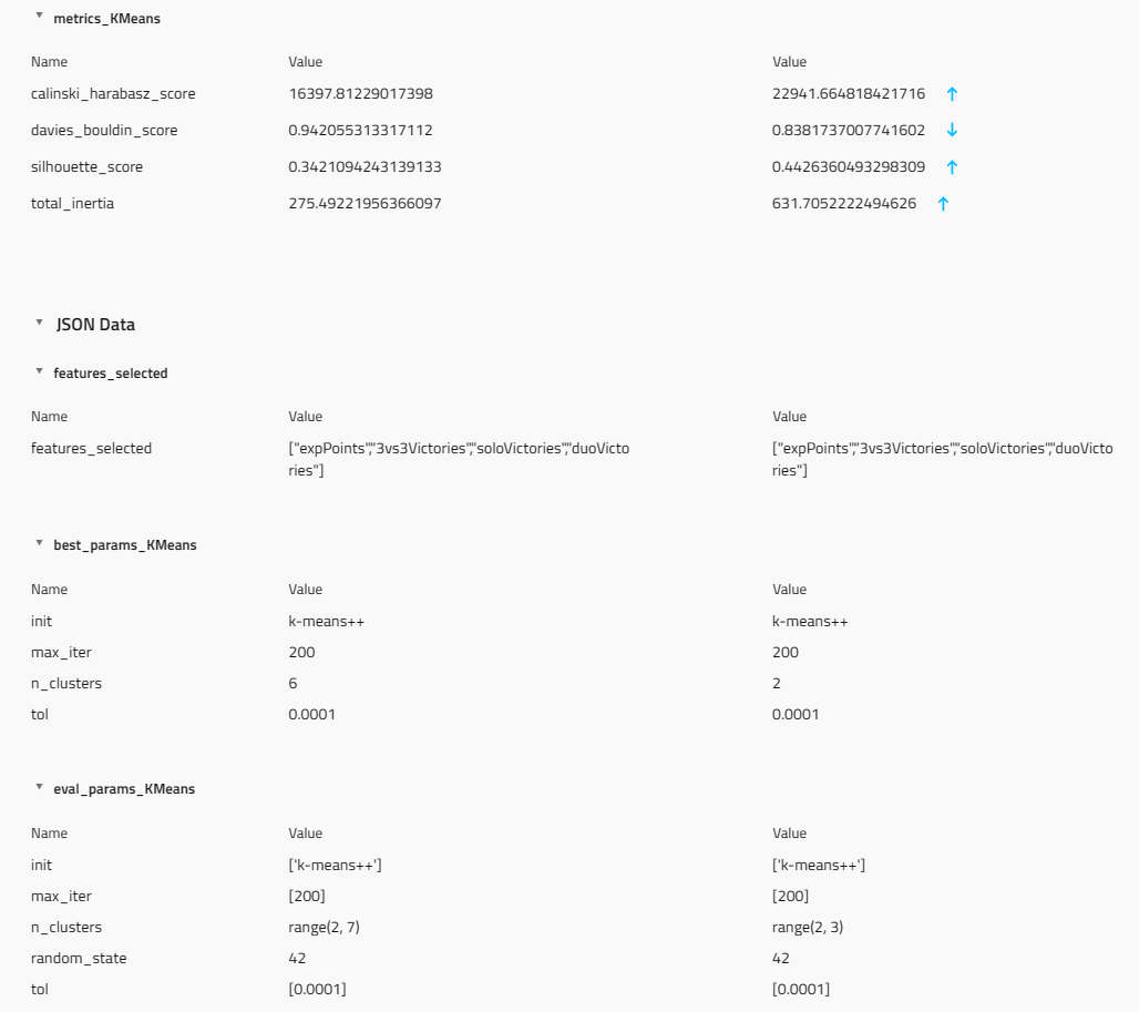
All of these metrics will be saved in the metrics_KMeans output, which will be saved as a model artifact and also versioned in our GCP model registry. This way, you will be able to visualize the experiment tracking in the Kedro Experiments section, as shown below.

This will allow you to track the performance of the model over time and identify any areas that need improvement.

Node: centroid_plot_generator_node

  1
  2
  3
  4
  5
  6
  7
  8
  9
 10
 11
 12
 13
 14
 15
 16
 17
 18
 19
 20
 21
 22
 23
 24
 25
 26
 27
 28
 29
 30
 31
 32
 33
 34
 35
 36
 37
 38
 39
 40
 41
 42
 43
 44
 45
 46
 47
 48
 49
 50
 51
 52
 53
 54
 55
 56
 57
 58
 59
 60
 61
 62
 63
 64
 65
 66
 67
 68
 69
 70
 71
 72
 73
 74
 75
 76
 77
 78
 79
 80
 81
 82
 83
 84
 85
 86
 87
 88
 89
 90
 91
 92
 93
 94
 95
 96
 97
 98
 99
100
101
102
103
104
105
106
107
108
109
110
111
112
113
114
115
116
117
118
119
120
121
122
123
124
125


def centroid_plot_generator(
    metadata_reduced: pd.DataFrame,
    kmeans_estimator: Union[bytes, None],
    parameters: Dict[str, Any],
) -> Tuple[go.Figure, go.Figure, go.Figure, go.Figure]:
    """
    Generate scatter plot figures for all possible pairs of features using the
    input metadata features (reduced, features selected), highlighting the centroids
    of a KMeans clustering estimator with the best hyperparameters found.
    Args:
        metadata_reduced: DataFrame containing the reduced metadata to be
        used for plotting
        kmeans_estimator: The KMeans clustering model to be used to generate the
        centroids
        parameters: A dictionary of parameters used to configure the plot dimensions
    Returns:
        Plot figures, where each plot shows a different pair of features in the input
        dataset, highlighting the centroids of the KMeans clustering model with the best
        hyperparameters found.
    """
    # Extract dimension parameters for plotting
    plot_dimensions = parameters.get("plot_dimensions")

    # Drop the 'player_id' column from the 'metadata_reduced' dataframe
    X_features = metadata_reduced.drop(columns=["player_id"])

    # Create a dictionary of feature names and their index in the feature matrix
    features = {
        X_features.columns[feature_number]: feature_number
        for feature_number in range(len(X_features.columns))
    }

    # Generate a list of all possible feature pairs
    feature_pairs = [
        (i, j) for i in range(len(features)) for j in range(i + 1, len(features))
    ]

    # Create an empty dictionary to store the plot figures
    plot_figures = {}

    # Iterate over each feature pair and create a plot figure for each pair
    for col_x, col_y in feature_pairs:
        log.info(f"Generating plot for features: {col_x} vs {col_y}")
        # Add some noise to the feature matrix
        noise = np.random.normal(loc=0, scale=0.05, size=X_features.shape)

        # Fit a KMeans model with the best hyperparameters found
        kmeans_estimator.fit(X_features + noise)

        # Get the coordinates of the centroids
        centroids = kmeans_estimator.cluster_centers_
        centroids_x = centroids[:, col_x]
        centroids_y = centroids[:, col_y]

        # Get the names of the two features being plotted
        feature_x = list(features.keys())[col_x]
        feature_y = list(features.keys())[col_y]

        # Get the values of the two features being plotted
        xs = X_features[feature_x]
        ys = X_features[feature_y]

        # Get the cluster labels for each data point
        labels = kmeans_estimator.labels_

        # Generate a palette of colors for the clusters
        colors = _generate_palette(kmeans_estimator.n_clusters)

        # Assign a color to each data point based on its cluster label
        point_colors = [colors[label % len(colors)] for label in labels]

        # Create a plot figure with two scatter traces: one for the data points and one
        # for the centroids
        fig = go.Figure()
        fig.add_trace(
            go.Scatter(
                x=xs, y=ys, mode="markers", marker=dict(color=point_colors, size=5)
            )
        )
        fig.add_trace(
            go.Scatter(
                x=centroids_x,
                y=centroids_y,
                mode="markers",
                marker=dict(
                    symbol="diamond",
                    size=10,
                    color=colors,
                    line=dict(color="black", width=2),
                ),
            )
        )

        # Add axis labels to the plot
        fig.update_layout(
            xaxis_title=f"{feature_x} scaled", yaxis_title=f"{feature_y} scaled"
        )

        # Set the size of the plot figure
        fig.update_layout(
            width=plot_dimensions.get("width"), height=plot_dimensions.get("height")
        )

        # Hide the legend in the plot
        fig.update_layout(showlegend=False)

        # Set the name of the plot figure and store it in the dictionary
        plot_name = f"{feature_x}_vs_{feature_y}"
        plot_figures[plot_name] = fig

    # Retrieve list of plot names as list
    plot_figures_names = list(plot_figures.keys())

    try:
        assert len(plot_figures_names) >= 4
        return (
            plot_figures[plot_figures_names[0]],
            plot_figures[plot_figures_names[1]],
            plot_figures[plot_figures_names[2]],
            plot_figures[plot_figures_names[3]],
        )
    except AssertionError:
        log.info("To save the plot figures the minimum number of plots must be 4")
        fig = _dummy_plot(plot_dimensions)
        return fig, fig, fig, fig

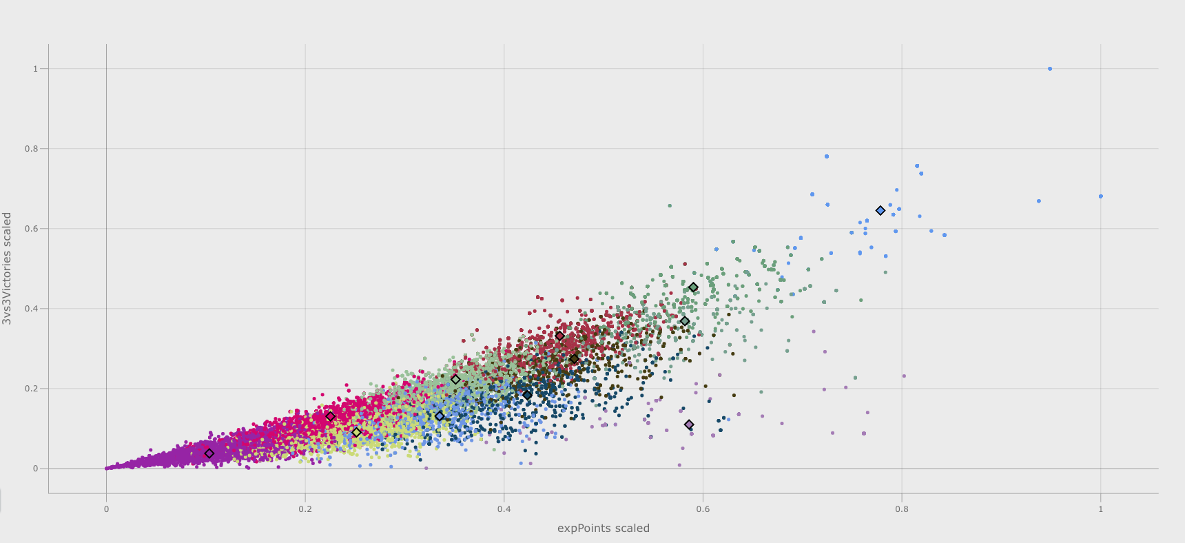
Finally, this node will generate visualizations of the centroids for each combination of X and Y variables. The plot below provides an example, where the centroids are represented by black-bordered squares.

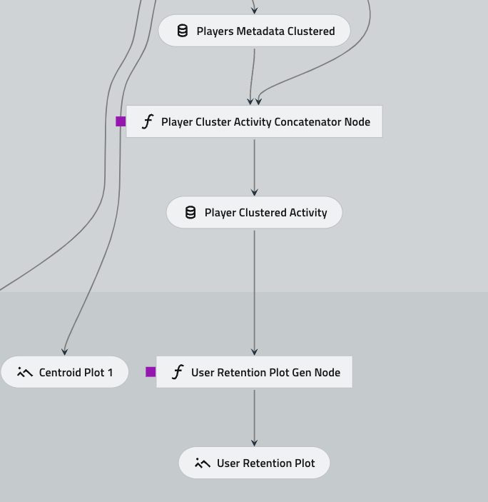
📊 Player activity data and Cluster labels merge Pipeline

Pipeline player_activity_clustering_merge

 1
 2
 3
 4
 5
 6
 7
 8
 9
10
11
12
13
14
15
16
17
18
19
20
21
22
23
24
25
26
27
28
29
30
31
32
33
34
35
36
37
38
39
40
41
42
43
44
45
46
47
48
49
50
51
52
53
54
55
56
57
58
59
60
61
62
63
64
65
66
67
68
69
70
71
72
73
74
75
76
77
78
79
80
81
82
83
84
85
86
87
88
89
90


def player_cluster_activity_concatenator(
    user_activity_data: pyspark.sql.DataFrame,
    players_metadata_clustered: pd.DataFrame,
    params_ratio_register: Dict[str, Any],
    params_activity_transformer: Dict[str, Any],
) -> pd.DataFrame:
    """
    Concatenates player clusters with their respective activity record activity data
    and calculates retention ratios based on provided analytical ratios.
    Args:
        user_activity_data: Spark DataFrame containing user retention data.
        players_metadata_clustered: DataFrame containing player data and cluster labels.
        params_ratio_register: Dictionary with ratio register parameters.
        params_activity_transformer: Dictionary with activity transformer parameters.
    Returns:
        Pandas DataFrame containing concatenated player cluster activity data and
        retention ratios
    """
    # Call | Create Spark Session
    spark = SparkSession.builder.getOrCreate()

    # Create Spark DataFrame from Pandas DataFrame
    players_metadata_clustered = spark.createDataFrame(
        data=players_metadata_clustered
    ).select("player_id", "cluster_labels")

    # Join user activity data with player metadata and cluster labels
    player_clustered_activity = user_activity_data.join(
        players_metadata_clustered, on="player_id", how="left"
    )

    # Select retention metric columns and dates of first log records
    ret_columns = player_clustered_activity.select(
        player_clustered_activity.colRegex("`^D\d+R$`")
    ).columns
    player_clustered_activity = player_clustered_activity.select(
        *["player_id", "cluster_labels", "first_log", *ret_columns]
    )
    # Group by cluster labels and first log date, and aggregate retention metrics
    player_clustered_activity = player_clustered_activity.groupBy(
        ["cluster_labels", "first_log"]
    ).agg(*[f.sum(col).alias(f"{col}") for col in ret_columns])

    # Get analytical ratios, normal ratios and days available from parameters,
    # and validate that all day labels are present
    analytical_ratios = [
        literal_eval(ratio) for ratio in params_ratio_register.get("analytical_ratios")
    ]
    ratios = [literal_eval(ratio) for ratio in params_ratio_register["ratios"]]
    days_available = params_activity_transformer.get("retention_days")

    # Convert retention metrics to percentages
    for ratio in ratios:
        num, den = ratio
        ratio_name = f"D{num}R"
        ret_num = f"D{num}R"
        ret_den = f"D{den}R"
        player_clustered_activity = player_clustered_activity.withColumn(
            ratio_name, ratio_agg(f.col(ret_num), f.col(ret_den))
        )

    # Obtain analytical ratios if them were defined in the parameters (ratio register)
    if params_ratio_register["analytical_ratios"] and isinstance(
        params_ratio_register["analytical_ratios"], list
    ):
        # Validate day labels are present in parameters
        _ratio_days_availabilty(analytical_ratios, days_available)

        # Calculate retention ratios for each analytical ratio (inputs)
        for ratio in analytical_ratios:
            num, den = ratio
            ratio_name = f"D{num}/D{den}"
            ret_num = f"D{num}R"
            ret_den = f"D{den}R"
            player_clustered_activity = player_clustered_activity.withColumn(
                ratio_name, ratio_agg(f.col(ret_num), f.col(ret_den))
            )

    # Reorder dataframe, reformat the cluster labels and send to data to driver
    player_clustered_activity = (
        player_clustered_activity.orderBy(f.asc("first_log"), f.asc("cluster_labels"))
        .dropna(subset=["cluster_labels"])
        .withColumn("cluster_labels", f.col("cluster_labels").cast("integer"))
        .toPandas()
    )

    # Present all installations as 100% retention
    player_clustered_activity["D0R"] = float(1.0)

    return player_clustered_activity

The purpose of the upcoming pipeline is to streamline the process of augmenting the retention data generated by the activity_transformer_node. Specifically, this involves incorporating the tags and cluster labels obtained from the output produced by the kmeans_inference_node. The ultimate objective is to utilize this enriched dataset to generate compelling visualizations through the user_retention_plot_gen_node.

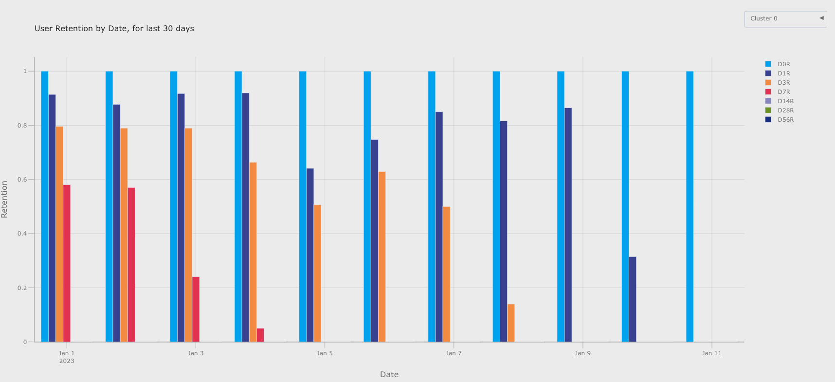
To illustrate the capabilities of this pipeline, let’s examine an example of the plots it can generate.

The cohort window displays the bounded retention data for players belonging to “Cluster 0”. Among users who installed the game by January 1st, 2023, the analysis reveals that 87% returned after the first day, 78% returned after the third day, and 56% of them continued engagement after the seventh day. It is important to note that these results are intended solely for demonstrative purposes, as they may be subject to bias due to the data collection method employed.

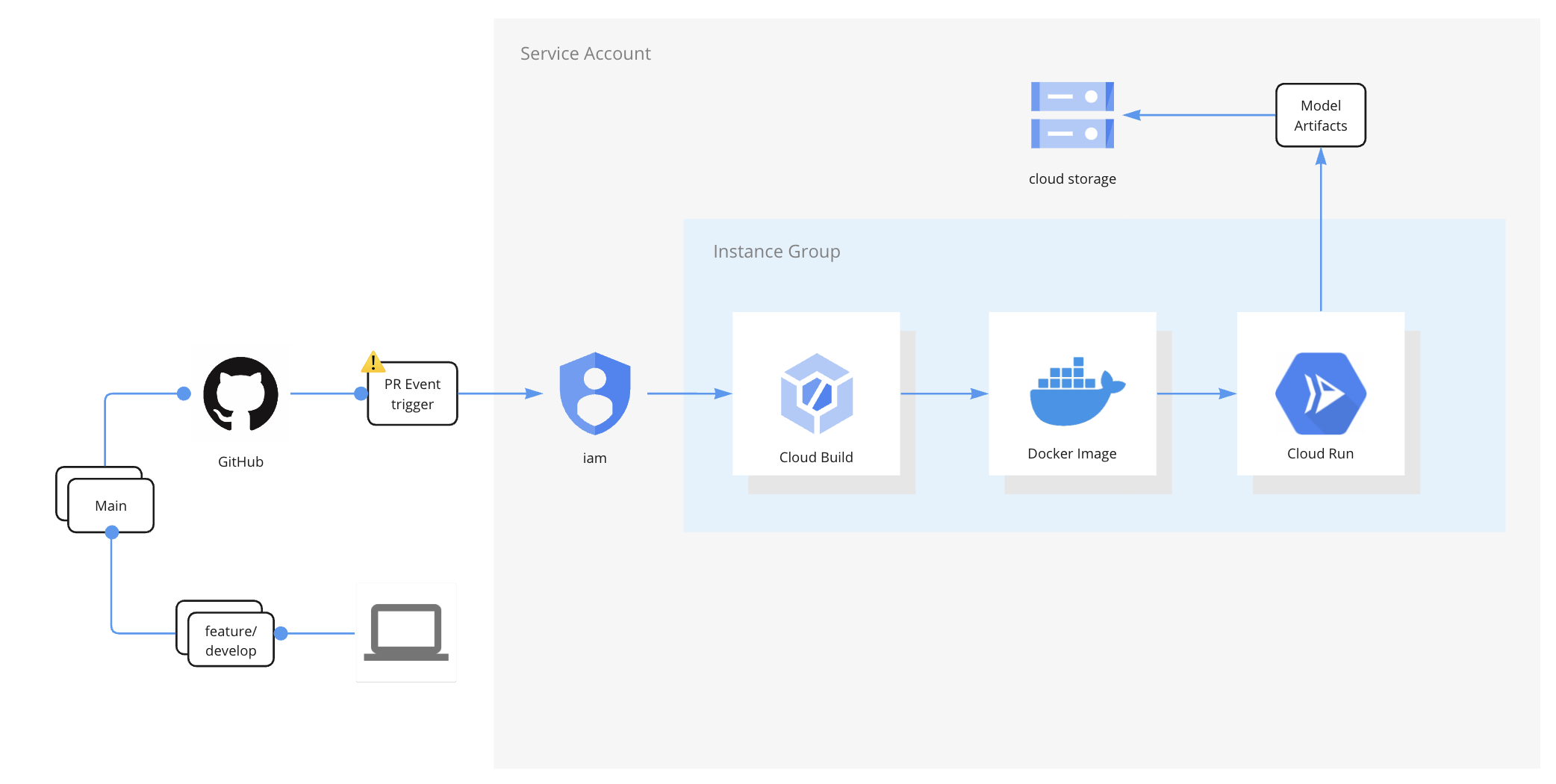
🌐 Deployment Demo

The deployment will be structured in a simple way to define an architecture that can run the job without complex services. In this case, I used a stateless service to run the job. The tech stack used is composed of the following elements:

GitHub repository: The code repository containing the code assembled as a Kedro project framework. This repository has two branches: one for development (feature/develop) and another for deployments (main).
Docker container: A container created with a Dockerfile that installs Java v8, Hadoop 3.1.1, and Spark 3.3.1 on top of a base image in Python 3.9. The container then executes the main CMD command to run the job.
Google Cloud Bucket: A place to store the raw data, staging data, and model artifacts. The bucket is structured to provide more traceability to the experiments.
Google Cloud Build: A service used for continuous development. When a user makes a pull request from the feature/develop branch to the main branch, an action is triggered in Google Cloud Build to rebuild the image based on the new code version.
Google Cloud Run: A computing platform with scalable infrastructure where the execution command is pointing, using the code image provided by the Cloud Build service.

Note that the execution of the code is pointing to the visualization command, that’s why the outputs are not loaded. This is because the main purpose of this deployment is to showcase this project. However, for a deployment on GCP, it is simple to change the CMD command at the end of the Dockerfile.

Additionally, the deployment was made public for this showcase using Google’s Free Program, and a VPC was not set up to let you access the pipeline view.

🗒️ Final thoughts & takeaways

What can the stakeholders understand and take into consideration?

Implementing an automated and parametrized pipeline for bounded retention metrics allows for focused analysis of player engagement and behavior, providing actionable insights for game improvement.

Real-time and reliable data enables designers to identify trends, patterns, and potential issues affecting customer retention, facilitating the implementation of targeted strategies and interventions.

What could the stakeholders do to take action?

Planning the data processing method is crucial to assess scalability and long-term parallelization technologies, minimizing risks and optimizing resource allocation.

Establishing a robust monitoring system helps track key metrics and performance indicators before and after new season releases, aiding in the identification of potential data drift sources.

Implementing good practices in Continuous Development allows for seamless productionalization of new changes and facilitates testing and deployment.

To compare different modeling strategies, A/B testing can be used by assembling new nodes to alternative versions of the same pipeline.

What can stakeholders keep working on?

Centralizing the solution into a single cloud provider, like Google Cloud Services, minimizes tech debt, simplifies management, and optimizes resource allocation and cost management.

Leveraging tools like Kedro, MLflow, and Neptune.ai for experiment tracking helps keep artifacts versioned and trackable over time, enhancing reproducibility and collaboration

ℹ️ Additional Information

Related Content

Here you have a list of preferred materials for you to explore if you’re interested in similar topics:

— Elite Game Developers Podcast by Joakim Achren.

— Joakim Achren’s newsletter and blog.

— Game Data Science book and additional info at the Oxford University Press.

— Getting started with Kedro.

— Brawlstats homepage, by overwolf.

Datasets

The extracted datasets will be uploaded to Kaggle as part of its public source intention.

Article disclaimer: The information presented in this article is solely intended for learning purposes and serves as a tool for the author’s personal development. The content provided reflects the author’s individual perspectives and does not rely on established or experienced methods commonly employed in the field. Please be aware that the practices and methodologies discussed in this article do not represent the opinions or views held by the author’s employer. It is strongly advised not to utilize this article directly as a solution or consultation material. ↩︎